Learning Locomotion
The Learning Locomotion project was a DARPA program with the goal of developing a new generation of learning algorithms to enable traversal of rough terrain by unmanned ground vehicles (UGV). Typically, UGVs are not capable of traversing rough terrain, limiting their available area of operation. This project looked to develop new control algorithms that employ advanced learning techniques in order to advance UGV capabilities in rough terrain.
The project had six research teams that both collaborate and compete. Each team was provided with the same small quadruped robot (Little Dog), built by Boston Dynamics. Each team was also provided with an advanced motion capture system by Vicon in order to reduce the complexity of sensing in the navigation problem. By using the same hardware, the research teams could focus on the problem of developing effective algorithms for negotiating rough terrain.
Detailed Description of Our Technical Approach
The highlights of our approach include the selection of salient state and action spaces, joint-trajectory free stance control, and effective teaching. The following description of our approach is from exerpts of our Learning Locomotion proposal written in April 2005.
Base Static Gait Algorithm
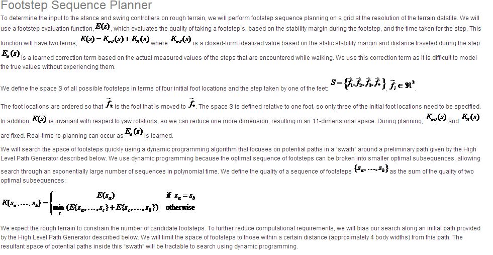
The first algorithm we develop will be a static one-leg-at-a-time crawl gait. We will use a divide-and-conquer approach, dividing the problem into the separate subtasks of stance control, swing control, terrain footstep mapping, and terrain quality mapping. For each subtask, we will implement a controller that uses a reduced degree-of-freedom, salient state and action space and learns a solution to the subtask while attempting to minimize a penalty function.
Stance Phase Controller
The input to the stance phase controller is the desired body center of mass position with respect to the center of the feet support polygon. The goal of the stance phase controller is to quickly get the robot from whatever configuration it is in to the desired center of mass position while maintaining stability. The desired orientation and height of the body will be determined based on the foot locations. The desired yaw will be that which makes the robot face forward; the desired pitch will be that which matches the slope of the ground, based on the foot locations; the desired roll will be zero; and the desired height will be a constant parameter. This choice is invariant throughout this controller and reduces the space of solutions.
The key feature of the stance phase controller is that we will transform the raw state and action spaces from joint positions, velocities, and torques to more salient, and reduced dimensional spaces. The transformed state vector will consist of: leg positions with respect to the center of the feet support polygon; body center of mass location and velocity with respect to the center of the feet support polygon; body pitch and roll; and pitch and roll velocities. The action vector will consist of the net vertical force from the legs, the net torques about the yaw, pitch, and roll axes, and the commanded center of pressure x and y location with respect to the center of mass. The yaw variables will be eliminated through a rotational transformation as the heading of the robot is irrelevant to the task of stance control. This leaves a state vector with 16 dimensions (18 when four legs are on the ground) and an action vector with 6 dimensions.
Since this is a large space, we will further divide the stance controller into subtasks of controlling body height, body orientation, and body x-y position. The height controller will use only body height as its state vector, vertical force as its action vector, and squared error between height and desired height as its penalty function to be minimized. The orientation controller will use support polygon pitch and body yaw, pitch, and roll and their derivatives as the state vector, net body torques as the action vector, and sum of the squared error between the desired orientation and the actual orientation as the penalty function to be minimized. The body x-y controller will have as the state vector the leg (x,y) positions and the body center of mass (x,y) location and velocity with respect to the center of the support polygon. It will use the center of pressure location with respect to the center of mass as the action vector. The penalty function will consist of the squared error between the desired and actual center of mass location, as well as a penalty for a low stability margin. The stability margin will be computed as the amount of sideways force that needs to be applied to the center of mass before it tips.
Each of the stance controller subtasks will be learned using a standard temporal difference Reinforcement Learning algorithm, such as Q-Learning with value function approximation. Learning will occur first on a simulation of the robot, initialized with randomly selected foot locations, body position, and body orientation. In simulation, we will run on the order of 1 million episodes until the algorithm reliably performs stance control. The resultant learned value function will then be transferred to the real robot where learning will continue. We will present the robot with a large number of training examples consisting of varying leg positions and desired body position. The leg positions will be set simply by setting the robot on different parts of the Terrain Board and the desired body positions will be randomly generated.
The described stance phase controller should be successful due to our state representation and a sensible division of subtasks. It will be tractable since the highest state dimension is 10 for the x-y position subtask.
Swing Leg Controller
The swing leg controller will have as its input the desired footstep location of the swing leg and a bounding sphere of keep-out regions for the leg, representing the ground protrusions that need to be avoided. The state vector will be the Cartesian position and velocity of the foot with respect to its hip location. The action vector will be the Cartesian forces on the foot. We will use a standard Reinforcement Learning algorithm with the penalty function to minimize consisting of the squared error between the desired foot location and the actual foot location, and the sum of the squared Cartesian forces on the foot endpoint.
As with the stance controller, we will first perform a significant amount of training in simulation and then transfer the learned behavior to the real robot for further training. After this learning, the swing leg controller will be able to quickly swing the leg to the desired location while avoiding the keep-out region. Further learning will lead to reduced swing time and hence quicker walking speed.
Justification of Our Approach
Our approach to Learning Locomotion will be successful due to its use of salient state and action spaces, a divide-and-conquer approach with subtasks and subgoals, choosing reduced dimensional state and action subspaces for each subtask, and by providing relevant training examples.
Similar reductions of spaces are typical in non-trivial examples of machine learning. The theoretical alternative is given the state of the Little Dog robot (joint angles and velocities), the state of the world (terrain map), and the goal (get to the other end of the Terrain Board), one could use pure tabular-based Reinforcement Learning to find the optimal action (servo commands) given the current state. This is a well posed reinforcement learning problem with textbook techniques that guarantee convergences. However, there are several “curses” that make this “Pure Reinforcement Learning” approach impossible. As with nearly all successful examples of nontrivial machine learning, we can “break” these curses using prior knowledge of the problem, human intuition, and approximation. The art is to determine the best way to incorporate these features without significantly degrading the solution quality.
Curse of Dimensionality. If we were to discretize each of the 12 joint angles, 12 joint velocities, and 3 orientation angles and velocities into only 10 discrete values, there would be 1030 states of the robot! This search space is too large to exhaustively search. To break the curse of dimensionality we will focus on promising regions of the state space, reduce the search space through the use of salient features as state variables, use approximation functions for generalization across regions of state space, and accept suboptimal but good solutions.
Needle in a Haystack Curse. In the space of control systems, the quantity of good controllers is very small compared to the quantity of all possible controllers. For systems such as legged robots, in which all bad controllers are equally bad with respect to the goal (how does one compare which of two robots fell down “better”?), the small subset of good controllers lives on “fitness plateaus” in the search space. Finding these plateaus can be a “needle in a haystack” problem. To break the needle in a haystack curse, we will guide learning onto plateaus in fitness space by providing examples, seeding learning routines, and narrowing the range of potential policies through the choice of control system structure.
Curse of Delayed Rewards with a Complex Task. The goal of the Learning Locomotion competition is to traverse the Terrain Board as quickly as possible. Thus no reward is given (and thus no learning occurs) in the pure Reinforcement Learning approach until a very complex sequence of actions is accomplished purely as a matter of chance. Crossing the board by pure chance would eventually occur theoretically, but with the complexity of this problem it would take a prohibitively long amount of time. To break the curse of delayed rewards, we will divide the problem into subtasks, provide intermediate rewards for partial work towards a goal, and seed value functions through examples.
Curse of the Expense of Real World Trials. The time cost of performing exploratory actions on a real robot is high. If each trial takes one minute, even a fully automated system can only perform 1440 trials per day. One cannot afford to waste these precious trials on unguided pure Reinforcement Learning in massive state spaces. To break the curse of the expense of real world trials, we will run numerous trials in simulation, and focus on potentially good solutions without exhaustive exploration of all possibilities.
In deciding which elements of expert knowledge to incorporate in the design of the learning algorithm, one must make a tradeoff between reducing the time to find a good solution in the reduced space of possibilities and reducing the potential optimality of solutions. Incorporating those elements of human knowledge that are fundamental to the problem of quadrupedal locomotion will have the greatest cost-benefit. Restrictions that are incorporated simply to make the problem tractable, or based on misconceptions of the quadrupedal locomotion problem would have the least cost-benefit. The trick is recognizing the difference and being masterful in the most appropriate incorporation of the most fundamental domain knowledge.
Divide and Conquer Approach
Quadrupedal animals smoothly transition from walk to trot to gallop gaits as speed increases. It is still debated whether a single mechanism accounts for each gait, or if there are several different mechanisms that are discretely switched as the gait changes. From an engineering point of view, the latter case allows for a system that is much easier to implement and will be the approach we take. We will develop separate learning algorithms for the crawl gait, trot walking, trot running, bounding, and jumping. The leg phasing for each gait will either be dictated by the controller structure or by penalizing non-conforming motion in reward functions.
Previous work on legged locomotion has shown that dividing the problem into subtasks, each with an independent controller can result in successful locomotion, even though the dynamics are coupled. The most widely known example of this approach is Raibert’s “three part controller”, in which height, pitch, and speed are controlled by separate individual control laws. In our work, we have utilized a similar approach, but have extended it by a) using multiple interacting controllers for some parts, such as speed control, and b) increasing the region of convergence by augmenting the decoupled controllers with coupled controllers that were either hand-crafted or generated through machine learning techniques. In this project we will use a separate learning algorithm to optimize each subtask. The subtasks will be defined through the state and action selection and the reward function for each learning algorithm. Each of these algorithms will be learning simultaneously and interact with each other. As one improves on its subtask, the others will be exposed to that change and improve upon their subtask accordingly.
Learning Locomotion Software
Body Localized Motion Capture: One improvement made on the motion capture data is the addition of Locap, which uses only the top six motion capture points on the dog to determine body position and orientation. Currently the motion capture determines body pose using all of the mocap points, making the position susceptible to the flakier leg mocap points. The top six points are seen by more cameras and therefore generally more reliable, yielding a better measure of body pose. In addition, the algorithm is robust to lost body points and flipped body points (when the mocap system momentarily switches the order of the points).
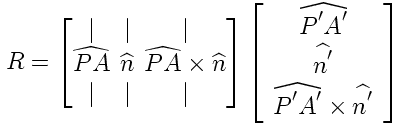
From the motion capture definition of the little dog robot, we can get a template of the 6 mocap markers in relation to the body center point at 0,0,0 position and orientation. Given any three of these points in the world (as observed during a run), we can find a transformation from the template trio (A’B’C’) to the world trio (ABC). First define the centroids P and P’ and the unit vectors shown below.
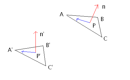
The rotation matrix from template space to world space is then:
translating the space to make the centroids coincident yields the transformation matrix
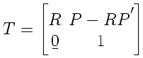
This 4×4 matrix can then be applied to the original template body center to get the position and orientation of the body according to the measured world trio. This algorithm is repeated for every set of three in the 6 body points, and the largest clump is averaged to yield the final Locap pose. The number of points in the clump can then be used as a measurement validity check.
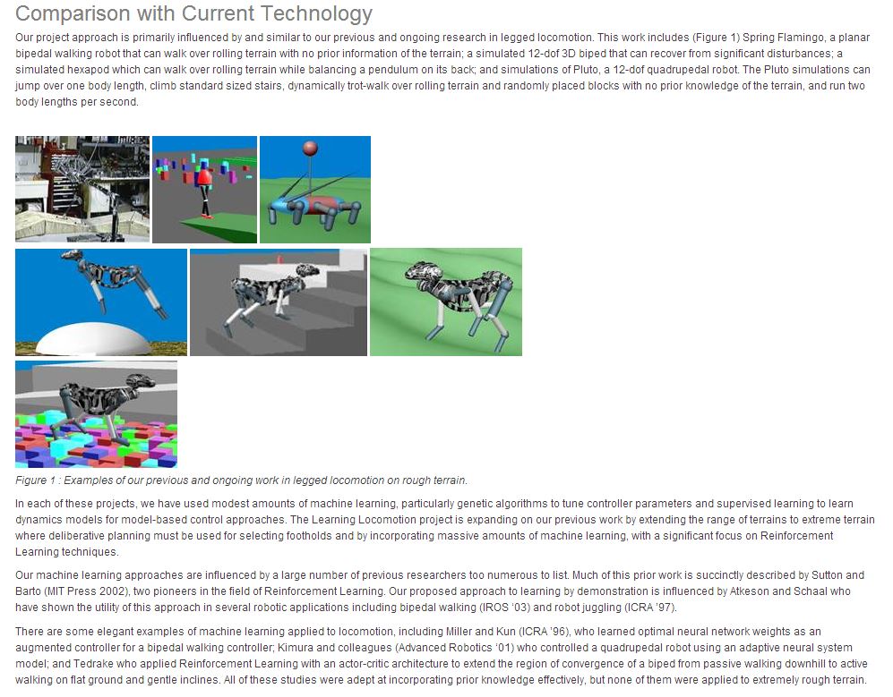
Learning Locomotion Publications
Related Publications
Learning Locomotion Data
Research Projects:
- Humanoid Robots as Human Avatars
- Nadia Humanoid
- Exoskeleton for Improving Mobility
- Cybathlon 2020
- Quadrupedal Locomotion
- Open Source Initiative
Past Projects:
- DARPA Robotics Challenge
- M2V2 Humanoid
- Learning Locomotion
- X1 Mina Exoskeleton
- Cybathlon 2016
- The Grasshopper
- FastRunner
IHMC Research Team:
- Jerry Pratt
- Peter Neuhaus
- Brian Bonnlander
- John Carff
- Travis Craig
- Divya Garg
- Johnny Godowski
- Greg Hill
- Tim Hutcheson
- Matt Johnson
- Carlos Perez
- John Rebula
- R. Sellaers
- S. Tamaddoni
- John Taylor